From architecture to fine-tuning, inference, and evaluation with MedGemma 1.5.
1Faculty of Applied Science and Engineering, University of Toronto · 2Princess Margaret Cancer Centre & AI Hub, University Health Network
Multimodal LLMs combine images, text, video, and audio in a single model - and they are rapidly becoming practical tools in clinical workflows. This mini course walks through the complete pipeline for a medical image-text-to-text task: understanding how MLLMs align modalities, dissecting the MedGemma 1.5 architecture, then preparing the FLARE-MLLM-2D dataset, fine-tuning with QLoRA, running inference, and evaluating report generation with CRIMSON and GREEN scores.
Every hands-on step runs in the linked interactive Jupyter notebook on Colab. This GitHub repository contains the course website; the executable notebook workflow remains on Colab.
By the end of this mini course you should be able to:
transformersFLARE-MLLM-2D and access to the MedGemma weights| 01 | BackgroundIntroduction to MLLM + clinical applications | Jump → |
| 02 | Model Architecture: MedGemma 1.5Detailed description of the model architecture | Jump → |
| 03 | Data PreparationPrepare the FLARE-MLLM-2D dataset for fine-tuning | Jump → |
| 04 | Fine-tuningFine-tune MedGemma 1.5 4B on the preprocessed dataset | Jump → |
| 05 | InferenceInfer with the base and fine-tuned MedGemma 1.5 4B | Jump → |
| 06 | EvaluationEvaluate MedGemma 1.5 4B’s performance on report generation using CRIMSON score and GREEN score | Jump → |
| 07 | ConclusionSummary of what we have covered in the mini course | Jump → |
| 08 | QuizTest your knowledge with the provided NotebookLM | Jump → |
Module 01
Introduction to MLLM + clinical applications.
MLLM emphasizes the alignment of latent spaces between different modalities. The building blocks are familiar - an image encoder and a text decoder - and the interesting question is how to combine encoders and decoders of different modalities so they can operate as one model.
Based on the input and output modalities, we can classify MLLMs into categories like the ones on the right. Hugging Face also uses these categories.
A vision encoder and a language model do not naturally understand one another:
Align vision features to an existing LLM
Compress vision through learned queries
Inject vision through cross-attention
Train a unified multimodal autoregressive model
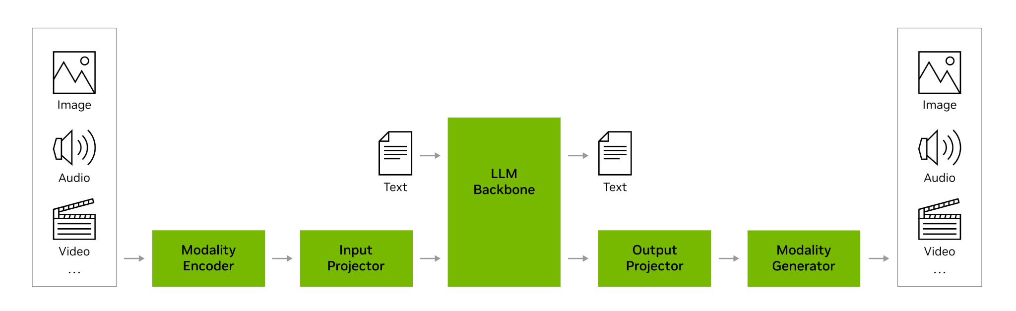
Figure credit: NVIDIA. (n.d.). Multimodal large language models. NVIDIA Glossary. Retrieved from nvidia.com/en-eu/glossary/multimodal-large-language-models · Extended reading: Multimodal Large Language Models - NVIDIA
MLLMs are powerful in a clinical workflow for perception, reasoning, documentation, triage, and patient-facing support.
Below are five concrete clinical applications (CAs), each illustrating one way an MLLM slots into practice.
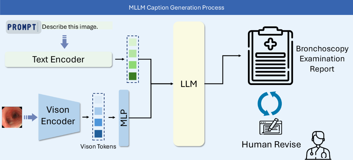
In a report generation task, the MLLM:
Figure credit: Luo, X., Huang, X., Liang, X. et al. Towards Automated Reporting: A Bronchoscopy Report Dataset for Enhancing Multimodality Large Language Models. Sci Data 13, 339 (2026). doi.org/10.1038/s41597-026-06692-8
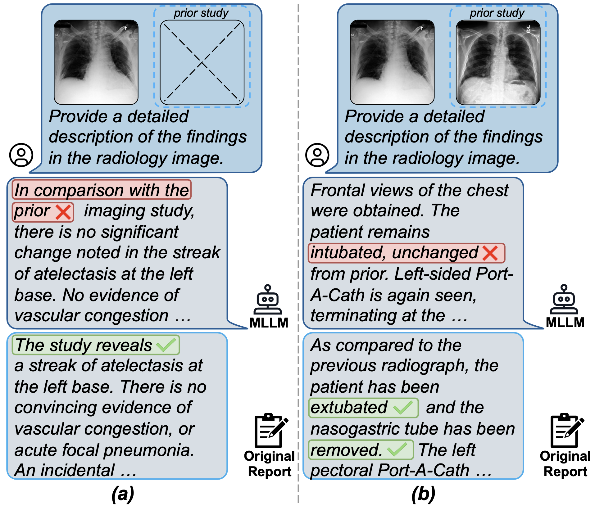
In a longitudinal comparison task, the MLLM:
Figure credit: Zhang, X., Meng, Z., Lever, J., & Ho, E. S. (2025, July). Libra: Leveraging temporal images for biomedical radiology analysis. In Findings of the Association for Computational Linguistics: ACL 2025 (pp. 17275–17303). doi.org/10.48550/arXiv.2411.19378
In a multi-class classification task, the MLLM outputs one label for several classes. It is the same as naive classification, but with outputs in the form of text - we use string parsers to convert the textual class ids into integers. Some common clinical examples are BI-RADS category, tumor subtype, disease stage, and dermatology diagnosis category.

Figure credit: Wikipedia - Cat (Cat_August_2010-4.jpg)
In a multi-label classification task, the MLLM outputs multiple labels at once. Common clinical examples include chest X-ray findings: edema, consolidation, atelectasis, cardiomegaly, and pleural effusion.
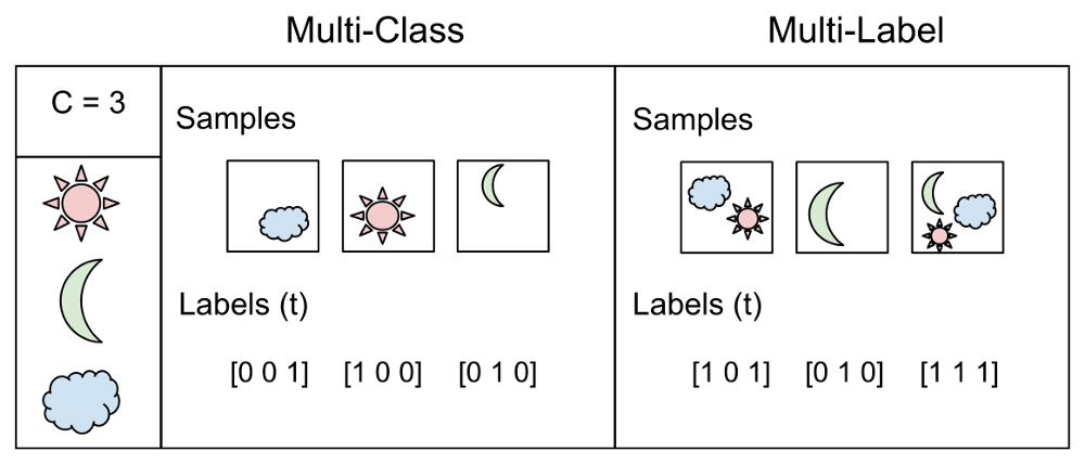
Figure credit: Sharma, G. (2021, February 7). Multi-label classification. Medium; Analytics Vidhya. medium.com/analytics-vidhya/multi-label-classification
In a regression task, the MLLM outputs a continuous value. It is the same as naive regression, but with outputs in the form of text - we use string parsers to convert the strings into floats. Some common clinical examples are ejection fraction, tumor size, organ volume, lab value prediction, risk score, and survival time.

Figure credit: Wikipedia - Cat (Cat_August_2010-4.jpg)
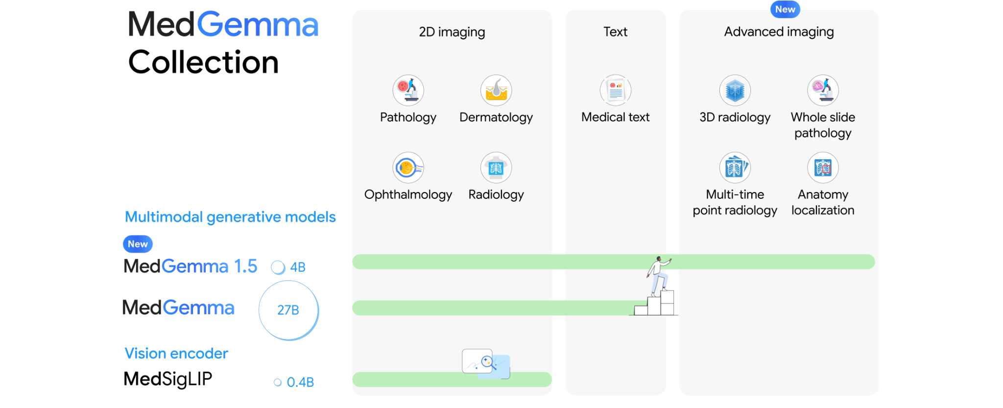
In this mini course, we are going to use MedGemma 1.5 4B as an example. The MedGemma family consists of LLaVA-style vision-language models (VLMs) designed for image-text-to-text tasks, specialized in medical images.
Throughout the mini course, we will be learning hands-on examples with MedGemma 1.5, covering a complete pipeline for the report generation task using the FLARE-MLLM-2D dataset.
Dataset: FLARE-MLLM-2D · Model: MedGemma 1.5 4B
Module 02
Detailed description of the MedGemma 1.5 model architecture.
Figure credit: Sellergren, A., Gao, C., Mahvar, F., Kohlberger, T., Jamil, F., Traverse, M., ... & Golden, D. (2026). MedGemma 1.5 technical report. arXiv preprint arXiv:2604.05081. doi.org/10.48550/arXiv.2604.05081
MedGemma 1.5 4B is based on Gemma 3 with the same general architecture, using a 400M MedSigLIP vision encoder as the visual front end and a decoder-only Transformer LLM as the text generator. Images are normalized to 896×896 and encoded into 256 visual tokens per image.
The key improvement between MedGemma 1 and MedGemma 1.5 is the long context window, with which we are able to feed multiple uniformly sampled slices (up to 85, modeled as a time sequence) to represent a 3D volume. However, in this mini course, we only deal with 2D images.
The encoder runs at a fixed 896×896 input and pools its 4,096 patch tokens down to 256 visual tokens. For images that are large or far from square, an optional “pan & scan” pass crops additional windows and encodes each one the same way, trading extra tokens for effective resolution.
Cited: Sellergren, A., Gao, C., Mahvar, F., Kohlberger, T., Jamil, F., Traverse, M., ... & Golden, D. (2026). MedGemma 1.5 technical report. arXiv preprint arXiv:2604.05081. doi.org/10.48550/arXiv.2604.05081
Module 03
Prepare the FLARE-MLLM-2D dataset for fine-tuning.
FLARE-MLLM-2D is a gated multimodal dataset for the MICCAI FLARE challenge. The course workflow selects its report-generation portion rather than downloading unrelated modalities. The complete collection is 35.6 GB, so a full download needs substantially more time and storage.
Since we use Hugging Face’s transformers as the backend of the pipeline, we want to convert the dataset format into Hugging Face’s supervised fine-tuning (SFT) records’ format.
The executable data-preparation workflow is in the interactive Colab notebook. The GitHub repository contains the supporting course website.
Module 04
Fine-tune MedGemma 1.5 4B on the preprocessed dataset.
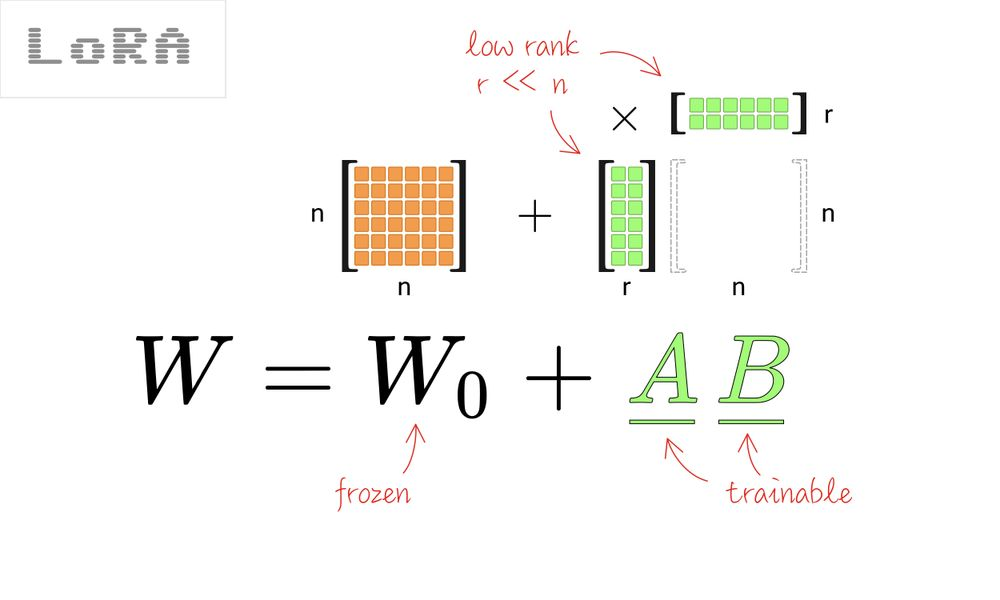
Even with foundation models trained on massive amounts of data, it is still extremely common that the application dataset is out of distribution (OoD). To adapt to the target domain, we need to apply fine-tuning. There are multiple ways to perform fine-tuning; in this mini course, we will focus on parameter-efficient fine-tuning (PEFT) - specifically QLoRA.
Figure credit: Görner, M. (2025, March 13). Are you still using LoRA to fine-tune your LLM? Towards Data Science. towardsdatascience.com/are-you-still-using-lora-to-fine-tune-your-llm
Method references: Hu, E. J., et al. (2021). LoRA: Low-Rank Adaptation of Large Language Models. · Dettmers, T., et al. (2023). QLoRA: Efficient Finetuning of Quantized LLMs.
In this mini course, we will fine-tune for only 0.25 epochs to save time.
Run fine-tuning in the interactive Colab notebook with a GPU runtime providing ≥ 40 GB VRAM (A100 or H100 class) - see Prerequisites for the full setup. The GitHub repository contains the supporting course website.
Module 05
Infer with the base and fine-tuned MedGemma 1.5 4B.
Now let us infer on 16 samples (to save time) in the validation set, with both the base and the fine-tuned model.
Run inference in the interactive Colab notebook with a GPU runtime providing ≥ 40 GB VRAM (A100 or H100 class) - see Prerequisites for the full setup. The GitHub repository contains the supporting course website.
Module 06
Evaluate MedGemma 1.5 4B’s performance on report generation using CRIMSON score and GREEN score.
Cited: Baharoon, M., Heintz, T., Raissi, S., Alabbad, M., Alhammad, M., AlOmaish, H., Kim, S. E., Banerjee, O., & Rajpurkar, P. (2026). CRIMSON: A clinically-grounded LLM-based metric for generative radiology report evaluation. arXiv preprint arXiv:2603.06183. doi.org/10.48550/arXiv.2603.06183
parse_error_counts in the green-score package); per-category counts and matched-finding counts land in a result dataframe.Cited: Ostmeier, S., Xu, J., Chen, Z., Varma, M., Blankemeier, L., Bluethgen, C., Michalson, A. E., Moseley, M., Langlotz, C., Chaudhari, A. S., & Delbrouck, J.-B. (2024). GREEN: Generative radiology report evaluation and error notation. In Findings of the Association for Computational Linguistics: EMNLP 2024 (pp. 374–390). Association for Computational Linguistics. doi.org/10.18653/v1/2024.findings-emnlp.21
Report-generation metrics inspect different signals, from exact wording to clinical error severity. This comparison is included for context; the hands-on notebook computes only GREEN and CRIMSON.
| Metric | What it compares | What it is useful for | Main limitation |
|---|---|---|---|
| BLEULexical | Exact candidate/reference n-gram precision, with a brevity penalty | Fast, reproducible comparison of wording overlap | Penalizes valid paraphrases and can barely react when one negation reverses a diagnosis |
| ROUGE-LLexical | Longest common subsequence between candidate and reference | Coverage and ordering of shared text | Measures surface similarity rather than factual or clinical correctness |
| BERTScoreSemantic | Token-level similarity using contextual embeddings | Recognizing paraphrases that use different wording | A general-language embedding match is not a direct test of findings, polarity, or clinical significance |
| CheXbert F1Clinical labels | Agreement on 14 observations extracted from chest X-ray reports | Checking high-level presence, absence, and uncertainty of common findings | Narrow chest X-ray label set; does not fully represent location, severity, measurements, or rare findings |
| RadGraph F1Clinical graph | Overlap of extracted radiology entities and relations | Comparing findings together with anatomy and selected relations | Depends on an information-extraction model and returns overlap rather than a direct explanation of clinical harm |
| RadCliQComposite | A learned combination of BLEU, BERTScore, CheXbert similarity, and RadGraph F1 | Predicting radiologist-assessed chest X-ray report error burden better than its individual components | Produces an opaque aggregate without identifying specific errors; raw RadCliQ variants are lower-is-better |
| GREENLLM judge | Matched findings plus six categories of significant and insignificant errors | Clinically aware scoring with a readable error explanation | Requires judge-model inference and inherits the judge’s scope and failure modes |
| CRIMSONLLM judge | Finding matches and attribute errors weighted by patient-specific clinical significance | Distinguishing minor errors from consequential omissions and hallucinations | Currently centered on chest X-ray reports and requires a configured judge plus clinical context |
Comparison framing follows the motivation and related-work discussion in Ostmeier et al. (2024), GREEN; descriptions are synthesized from the original metric papers linked above.
A single negation reverses the clinical meaning while leaving most words unchanged.
Adult patient; pleural effusion is a clinically relevant finding.
Pleural effusion present.
Pleural effusion not present.
| Metric | Example output | What the output reveals |
|---|---|---|
| BLEU | 0.75 | The score remains high because three of the four words overlap; the clinically decisive negation has little effect. |
| ROUGE-L | 0.57 | The shared word sequence dominates even though the diagnosis is reversed. |
| BERTScore | 0.75 | Contextual similarity drops, but the two nearly identical sentences still appear semantically close. |
| CheXbert F1 | 0.00 for the sole positive target finding | The extracted pleural-effusion label changes from positive to negative. A full 14-label micro- or macro-F1 also depends on how the remaining labels are aggregated. |
| RadGraph F1 | 0.50 | The finding entity overlaps, but its presence status does not, so the graph match receives only partial credit. |
| RadCliQ | Higher / worse error estimate | RadCliQ combines several component scores. There is no portable single-case number because v0/v1, checkpoints, normalization, and component implementations affect the output; raw variants are lower-is-better. |
| GREEN | 0.00 0 matched findings; 1 significant error |
The explanation identifies that pleural effusion is positive in the reference but negative in the generated report. |
| CRIMSON | 0.00 missing weighted finding; no earned credit |
Assuming pleural effusion is the only clinically weighted reference finding, its omission contributes to the denominator but earns no credit. Exact wording and weight depend on patient context and judge configuration. |
Reading the numbers. BLEU, ROUGE-L, BERTScore, RadGraph F1, and GREEN values are the published outputs for this pair in Figure 1 of the GREEN paper. CheXbert shows the finding-level F1 implied by the positive-to-negative label disagreement. The RadCliQ and CRIMSON rows are explicitly configuration-aware rather than fabricated point estimates.
CONTEXT: 78-year-old, dyspnea.
REFERENCE: Moderate left pleural effusion. Aortic atherosclerosis.
There is a moderate effusion in the left pleural space. Atherosclerotic aorta.
Shares few exact n-grams with the reference, so BLEU and ROUGE-L rank this report lower than the one on the right.
GREEN
2 / (2 + 0) → 1.00
CRIMSON
(0.5 − 0) / Wref = 0.5 / 0.5 → 1.00
No left pleural effusion. Aortic atherosclerosis.
Reuses the reference’s exact wording, so surface metrics score it higher - a one-word negation that inverts the diagnosis barely moves them.
GREEN
1 / (1 + 1) → 0.50
CRIMSON
(0 − 0) / 0.5 → 0.00
Errors come from six categories: false finding, missing finding, wrong location, wrong severity, a comparison absent from the reference, and an omitted prior-study comparison. The judge tags each one significant or insignificant, and only significant errors reach the denominator.
Every abnormal finding carries a rubric weight w, set with the patient’s age and indication in view:
C is the credit the candidate earns. Each matched finding contributes its own weight wi, scaled by a partial-credit factor that equals 1 when every attribute is right and shrinks as significant attribute errors (0.5 each) accumulate. Because wi sits in both numerator and denominator, one attribute error costs proportionally less on an urgent finding than on a minor one.
S is the raw score: net credit, C minus the weight of hallucinated findings Efalse, over Wref - the total significance available in the reference. Missing findings are penalized implicitly: they count toward Wref but earn no credit. Below zero the score is squashed by −A/(1+A), A = Efalse − C, so it approaches -1 asymptotically however many false findings pile up.
Let us evaluate the inference outputs using CRIMSON score and GREEN score.
The evaluation cell prints a per-sample table and a mean CRIMSON and GREEN score for both the base and the fine-tuned checkpoint, so you can compare them directly. Here is what to look for when your run finishes:
Do not read these numbers as a benchmark result. This run fine-tunes for 0.25 epochs and evaluates on 16 validation samples, both chosen so the notebook finishes in minutes. At that scale the difference between the base and fine-tuned means is well within noise, and a re-run can reverse the ordering. Evaluator configuration also matters: the official CRIMSON package defaults to MedGemmaCRIMSON, while an optional API-backed judge may introduce additional run-to-run variability. Treat the output as a demonstration that the pipeline is wired correctly end to end. For a result worth reporting, train at least one full epoch, evaluate the entire validation split, and record the exact evaluator and decoding settings.
Run evaluation in the interactive Colab notebook with a GPU runtime providing ≥ 40 GB VRAM (A100 or H100 class) - see Prerequisites for the full setup. The GitHub repository contains the supporting course website.
Module 07
Module 08
A NotebookLM has been prepared with the course materials - quiz yourself on everything covered in this mini course.
Open the NotebookLM QuizThis course builds on datasets, models, software, and educational resources created by the wider medical AI and open-source communities.
transformers conventions for model loading and supervised fine-tuning. Evaluation builds on the official green-score and crimson-score codebases.image-slot.js and tweaks-panel.jsx helpers are based on the Omelette starter scaffold included with the original site prototype; minicourse-tweaks.jsx supplies course-specific settings.The instructors reviewed and edited the AI-assisted outputs and remain responsible for the final tutorial. AI-generated material is not treated as a primary source; the papers, datasets, and software cited throughout the course provide the underlying references.
Figures and research claims are credited beside the relevant material throughout the course. Their inclusion does not transfer ownership; reuse remains subject to each original source’s terms.
Faculty of Applied Science and Engineering, University of Toronto · Princess Margaret Cancer Centre & AI Hub, University Health Network
Princess Margaret Cancer Centre & AI Hub, University Health Network